Tuesday, November 19, 2013

An example of exploratory analysis in R (lattice package)

Data Analysis Project 1

Introduction

Data set

The data consists of a sample of 2,500 peer-to-peer loans (= number of observations/samples) issued through the Lending Club. The interest rate of these loans is determined by the Lending Club on the basis of characteristics of the person asking for the loan such as their employment history, credit history, and credit worthiness scores. Such a data set (loansData.csv) is stored in working directory.
Let's load the data set and do some convenient operations aimed to traslate fake factor variables (e.g. Debt.To.Income.Ratio) into numeric variables.
data <- read.csv("loansData.csv")
data$MyInterest.Rate <- as.numeric(sub("%", "", data$Interest.Rate))/100
data$MyDebt.To.Income.Ratio <- as.numeric(sub("%", "", data$Debt.To.Income.Ratio))/100
doMean <- function(x) {
    ret <- vector("numeric", length = length(x))
    for (i in 1:length(x)) {
        ret[i] <- (as.numeric(substr(x[i], 1, 3)) + as.numeric(substr(x[i], 
            5, 7)))/2
    }
    ret
}
data$FICO.Range.mean <- doMean(data$FICO.Range)

Purpose of analysis

The purpose of analysis is to identify and quantify associations between the interest rate of the loan and the other variables in the data set. In particular, considering whether any of these variables have an important association with interest rate after taking into account the applicant's FICO score.

Methods and Results

Bivariate analysis

Let's start considering the association between Interest Rate and FICO range.
## par(mfrow=c(1,2))
plot(data$MyInterest.Rate, data$FICO.Range, pch = 19, col = "blue", cex = 0.5, 
    main = "Fig. 1 - The association between Interest Rate and FICO score range", 
    xlab = "FICO score range", ylab = "Interest rate")
plot of chunk unnamed-chunk-3
boxplot(data$MyInterest.Rate ~ data$FICO.Range, col = terrain.colors(length(data$FICO.Range), 
    alpha = 0.8), varwidth = TRUE, main = "Fig. 2 - The association between Interest Rate and FICO score range", 
    xlab = "FICO range score", ylab = "Interest rate")
plot of chunk unnamed-chunk-3
As showed by Fig. 1 and Fig. 2, Interest rate (quantitative response variable) seems negatively associated with FICO score range (categorical explanatory variable). In order to prove these variable are significantly (confidence level 95%) associated applying Pearson correlation, we consider the variable FICO score range mean (quantitative) instead of FICO score range (categorical).
cor.test(data$MyInterest.Rate, data$FICO.Range.mean, method = "pearson", conf.level = 0.95)
## 
##  Pearson's product-moment correlation
## 
## data:  data$MyInterest.Rate and data$FICO.Range.mean
## t = -50.26, df = 2498, p-value < 2.2e-16
## alternative hypothesis: true correlation is not equal to 0
## 95 percent confidence interval:
##  -0.7281 -0.6891
## sample estimates:
##     cor 
## -0.7091
Hence, we can conclude Interest rate is negatively associated with FICO score range mean (p-value < .0001). Moreover, if we know the FICO score range mean, we can predict 50,2% (Adjusted R-squared: 0.5026) of the variability we will see in Interest rate.
lm1 <- lm(data$MyInterest.Rate ~ data$FICO.Range.mean)
summary(lm1)
## 
## Call:
## lm(formula = data$MyInterest.Rate ~ data$FICO.Range.mean)
## 
## Residuals:
##      Min       1Q   Median       3Q      Max 
## -0.07988 -0.02136 -0.00455  0.01837  0.10195 
## 
## Coefficients:
##                       Estimate Std. Error t value Pr(>|t|)    
## (Intercept)           7.29e-01   1.19e-02    61.2   <2e-16 ***
## data$FICO.Range.mean -8.46e-04   1.68e-05   -50.3   <2e-16 ***
## ---
## Signif. codes:  0 '***' 0.001 '**' 0.01 '*' 0.05 '.' 0.1 ' ' 1
## 
## Residual standard error: 0.0295 on 2498 degrees of freedom
## Multiple R-squared:  0.503,  Adjusted R-squared:  0.503 
## F-statistic: 2.53e+03 on 1 and 2498 DF,  p-value: <2e-16
Are there other features statistically correlated to Interest rate explaining more variability than FICO range?
features = dim(data)[2]
pValue <- rep(NA, features)
r2 <- rep(NA, features)
for (i in 1:features) {
    lm1sum <- summary(lm(data$MyInterest.Rate ~ data[, i]))
    pValue[i] <- lm1sum$coeff[2, 4]
    r2[i] <- lm1sum$adj.r.squared
}

data.frame(names(data), pValue, r2)
##                       names.data.     pValue         r2
## 1                Amount.Requested  1.545e-65  0.1101018
## 2      Amount.Funded.By.Investors  1.326e-67  0.1134749
## 3                   Interest.Rate  0.000e+00  1.0000000
## 4                     Loan.Length 1.772e-109  0.1791880
## 5                    Loan.Purpose  1.654e-03  0.0322881
## 6            Debt.To.Income.Ratio  8.447e-01  0.0472510
## 7                           State  1.575e-02  0.0036624
## 8                  Home.Ownership  2.026e-01  0.0062175
## 9                  Monthly.Income  5.396e-01 -0.0002497
## 10                     FICO.Range  8.741e-01  0.5382865
## 11              Open.CREDIT.Lines  6.169e-06  0.0077580
## 12       Revolving.CREDIT.Balance  2.246e-03  0.0033351
## 13 Inquiries.in.the.Last.6.Months  1.216e-16  0.0267187
## 14              Employment.Length  3.751e-01 -0.0001105
## 15                MyInterest.Rate  0.000e+00  1.0000000
## 16         MyDebt.To.Income.Ratio  2.733e-18  0.0296123
## 17                FICO.Range.mean  0.000e+00  0.5026398
We found that several features are statistically correlated (confidence level 95%) to Interest rate but FICO range mean can predict its variability better than other variables. After FICO range, the features statistically correlated to Interest rate that predict best its variability are
  1. Loan.Length (18%)
  2. Amount.Funded.By.Investors (11%)
  3. Amount.Requested (11%)

Potential moderators

Such a negative association holds also for each loan purpose / with and without home ownsership / for each US state or do these variables moderate the association between Interest rate and FICO score?
library(lattice)
xyplot(data$MyInterest.Rate ~ data$FICO.Range.mean | data$Loan.Purpose, panel = function(x, 
    y, ...) {
    panel.xyplot(x, y, ...)
    lm1 <- lm(y ~ x)
    lm1sum <- summary(lm1)
    r2 <- lm1sum$adj.r.squared
    p <- lm1sum$coefficients[2, 4]
    panel.abline(lm1)
    panel.text(labels = bquote(italic(R)^2 == .(format(r2, digits = 3))), x = 780, 
        y = 0.15)
    panel.text(labels = bquote(italic(p) == .(format(p, digits = 3))), x = 770, 
        y = 0.2)
}, data = data, as.table = TRUE, xlab = "FICO range score mean", ylab = "Interest rate", 
    main = "Fig. 3 - Interest rate vs. FICO range (mean) score for each loan purpose")
plot of chunk unnamed-chunk-7
Looking at Fig. 3, we find that FICO scores explains better the variability of interest rate in case of loan for education (explain 75% variability, p < 0.001), vacation (explain 71% variability, p < 0.001), medical (explain 66% variability, p < 0.001), car (explain 61% variability, p < 0.001) and house (explain 60% variability, p < 0.001).
xyplot(data$MyInterest.Rate ~ data$FICO.Range.mean | data$Home.Ownership[data$Home.Ownership != 
    "NONE"], data = data, as.table = TRUE, panel = function(x, y, ...) {
    panel.xyplot(x, y, ...)
    lm1 <- lm(y ~ x)
    lm1sum <- summary(lm1)
    r2 <- lm1sum$adj.r.squared
    p <- lm1sum$coefficients[2, 4]
    panel.abline(lm1)
    panel.text(labels = bquote(italic(R)^2 == .(format(r2, digits = 3))), x = 780, 
        y = 0.15)
    panel.text(labels = bquote(italic(p) == .(format(p, digits = 3))), x = 770, 
        y = 0.2)
}, xlab = "FICO range score", ylab = "Interest rate", main = "Fig. 4 - Interest rate vs. FICO range with and without home ownership")
plot of chunk unnamed-chunk-8

xyplot(data$MyInterest.Rate ~ data$FICO.Range.mean | data$State[data$State != 
    "MS" & data$State != "MD" & data$State != "IA"], data = data, as.table = TRUE, 
    panel = function(x, y, ...) {
        panel.xyplot(x, y, ...)
        lm1 <- lm(y ~ x)
        lm1sum <- summary(lm1)
        r2 <- lm1sum$adj.r.squared
        p <- lm1sum$coefficients[2, 4]
        panel.abline(lm1)
        if (p > 0.001) {
            panel.text(labels = bquote(italic(p) == .(format(p, digits = 3))), 
                x = 770, y = 0.2)
        }
        panel.text(labels = bquote(italic(R)^2 == .(format(r2, digits = 3))), 
            x = 780, y = 0.15)

    }, xlab = "FICO range score", ylab = "Interest rate", main = "Fig. 5 - Interest rate vs. FICO range score for each US state")
plot of chunk unnamed-chunk-8
As showed, such a statistically significant negative association is confirmed also for each loan purpose / with and without home ownsership / for each US state. So, these variables don't moderate the association between Interest rate and FICO score.
Just a note regarding analisys by state: in some cases there'are not enough observations to estimate coefficents (MS,MD,IA), while in some other cases there're enough observations to calculate coefficients but we have p > 0.001. For instance, in case of SD there're just 4 obs.

Variables associated with interest rate at the same level of applicant's FICO score

data$FICO.Range.cut <- equal.count(data$FICO.Range.mean, 15)
xyplot(data$MyInterest.Rate ~ data$Monthly.Income | data$FICO.Range.cut, data = data, 
    as.table = TRUE, panel = function(x, y, ...) {
        panel.xyplot(x, y, ...)
        ## panel.loess(x,y)
        lm1 <- lm(y ~ x)
        lm1sum <- summary(lm1)
        r2 <- lm1sum$adj.r.squared
        p <- lm1sum$coefficients[2, 4]
        panel.abline(lm1)
        # panel.text(labels=x,x,y)
        panel.text(labels = bquote(italic(R)^2 == .(format(r2, digits = 3))), 
            x = 65000, y = 0.15)
        panel.text(labels = bquote(italic(p) == .(format(p, digits = 3))), x = 65000, 
            y = 0.2)
    }, xlab = "Montly Income", ylab = "Interest rate", main = "Fig. 6 - Interest rate vs. Montly Income in different FICO score levels")
plot of chunk unnamed-chunk-9


xyplot(data$MyInterest.Rate ~ data$Open.CREDIT.Lines | data$FICO.Range.cut, 
    data = data, as.table = TRUE, panel = function(x, y, ...) {
        panel.xyplot(x, y, ...)
        ## panel.loess(x,y)
        lm1 <- lm(y ~ x)
        lm1sum <- summary(lm1)
        r2 <- lm1sum$adj.r.squared
        p <- lm1sum$coefficients[2, 4]
        panel.abline(lm1)
        # panel.text(labels=x,x,y)
        panel.text(labels = bquote(italic(R)^2 == .(format(r2, digits = 3))), 
            x = 30, y = 0.15)
        panel.text(labels = bquote(italic(p) == .(format(p, digits = 3))), x = 30, 
            y = 0.2)
    }, xlab = "Credit lines", ylab = "Interest rate", main = "Fig. 7 - Interest rate vs. Credit lines in different FICO score levels")
plot of chunk unnamed-chunk-9


xyplot(data$MyInterest.Rate ~ data$MyDebt.To.Income.Ratio | data$FICO.Range.cut, 
    data = data, as.table = TRUE, panel = function(x, y, ...) {
        panel.xyplot(x, y, ...)
        ## panel.loess(x,y)
        lm1 <- lm(y ~ x)
        lm1sum <- summary(lm1)
        r2 <- lm1sum$adj.r.squared
        p <- lm1sum$coefficients[2, 4]
        panel.abline(lm1)
        # panel.text(labels=x,x,y)
        panel.text(labels = bquote(italic(R)^2 == .(format(r2, digits = 3))), 
            x = 0.2, y = 0.15)
        panel.text(labels = bquote(italic(p) == .(format(p, digits = 3))), x = 0.2, 
            y = 0.2)
    }, xlab = "Debt To Income Ratio", ylab = "Interest rate", main = "Fig. 8 - Interest rate vs. Debt To Income Ratio in diff. FICO score levels")
plot of chunk unnamed-chunk-9

histogram(~data$MyInterest.Rate | data$FICO.Range.cut, data = data, xlab = "Interest rate", 
    main = "Fig. 9 - Interest rate distribution across diff. FICO score levels")
plot of chunk unnamed-chunk-9

Missing data or other unusual features

There are 7 missing values in the provided data set.
sum(is.na(data))
## [1] 7
Regarding unusual features the list could be pretty long. Let's mention just the FICO score that is provided as factor variable and it's by grouped by range and it's not provided as numeric variable.

Potential confounders

Credit scores are designed to measure the risk of default by taking into account various factors in a person's financial history. Although the exact formulas for calculating credit scores are secret, FICO has disclosed the following components:
  • (30%) Credit utilization: the ratio of current revolving debt (such as credit card balances) to the total available revolving credit or credit. This components is probably correlated to Debt.To.Income.Ratio
  • (15%) Length of credit history. This components is probably correlated to Loan.Length
  • (10%) Types of credit used. This components is probably correlated to Loan.Purpose
  • (10%) Recent searches for credit. This components is probably correlated to Inquiries.in.the.Last.6.Months
All these hypotesis are true except the one regarding the correlation between Loan.Length and FICO score.
summary(lm(data$FICO.Range.mean ~ data$MyDebt.To.Income.Ratio))
## 
## Call:
## lm(formula = data$FICO.Range.mean ~ data$MyDebt.To.Income.Ratio)
## 
## Residuals:
##    Min     1Q Median     3Q    Max 
## -79.14 -26.61  -5.82  21.53 116.52 
## 
## Coefficients:
##                             Estimate Std. Error t value Pr(>|t|)    
## (Intercept)                   723.56       1.56   464.0   <2e-16 ***
## data$MyDebt.To.Income.Ratio  -101.92       9.11   -11.2   <2e-16 ***
## ---
## Signif. codes:  0 '***' 0.001 '**' 0.01 '*' 0.05 '.' 0.1 ' ' 1
## 
## Residual standard error: 34.2 on 2498 degrees of freedom
## Multiple R-squared:  0.0477, Adjusted R-squared:  0.0473 
## F-statistic:  125 on 1 and 2498 DF,  p-value: <2e-16
anova(lm(data$FICO.Range.mean ~ data$Loan.Length))
## Analysis of Variance Table
## 
## Response: data$FICO.Range.mean
##                    Df  Sum Sq Mean Sq F value Pr(>F)
## data$Loan.Length    1     459     459    0.37   0.54
## Residuals        2498 3066619    1228
anova(lm(data$FICO.Range.mean ~ data$Loan.Purpose))
## Analysis of Variance Table
## 
## Response: data$FICO.Range.mean
##                     Df  Sum Sq Mean Sq F value Pr(>F)    
## data$Loan.Purpose   13  179846   13834    11.9 <2e-16 ***
## Residuals         2486 2887233    1161                   
## ---
## Signif. codes:  0 '***' 0.001 '**' 0.01 '*' 0.05 '.' 0.1 ' ' 1
summary(lm(data$FICO.Range.mean ~ data$Inquiries.in.the.Last.6.Months))
## 
## Call:
## lm(formula = data$FICO.Range.mean ~ data$Inquiries.in.the.Last.6.Months)
## 
## Residuals:
##    Min     1Q Median     3Q    Max 
## -68.23 -28.23  -7.99  21.77 121.77 
## 
## Coefficients:
##                                     Estimate Std. Error t value Pr(>|t|)
## (Intercept)                          710.233      0.866  820.15   <2e-16
## data$Inquiries.in.the.Last.6.Months   -2.620      0.567   -4.62    4e-06
##                                        
## (Intercept)                         ***
## data$Inquiries.in.the.Last.6.Months ***
## ---
## Signif. codes:  0 '***' 0.001 '**' 0.01 '*' 0.05 '.' 0.1 ' ' 1
## 
## Residual standard error: 34.9 on 2496 degrees of freedom
##   (2 observations deleted due to missingness)
## Multiple R-squared:  0.00849,    Adjusted R-squared:  0.0081 
## F-statistic: 21.4 on 1 and 2496 DF,  p-value: 3.95e-06

A more powerful linear model

Let's build a multiple variable regression model with FICO range and other features statistically correlated to Interest rate that predict best its variability
  1. FICO Range mean (50%)
  2. Loan.Length (18%)
  3. Amount.Funded.By.Investors (11%)
  4. Amount.Requested (11%)
lm1sum <- summary(lm(data$MyInterest.Rate ~ data$FICO.Range.mean + data$Amount.Requested + 
    data$Amount.Funded.By.Investors + data$Loan.Length))
lm1sum
## 
## Call:
## lm(formula = data$MyInterest.Rate ~ data$FICO.Range.mean + data$Amount.Requested + 
##     data$Amount.Funded.By.Investors + data$Loan.Length)
## 
## Residuals:
##      Min       1Q   Median       3Q      Max 
## -0.09763 -0.01453 -0.00135  0.01271  0.10275 
## 
## Coefficients:
##                                  Estimate Std. Error t value Pr(>|t|)    
## (Intercept)                      7.26e-01   8.53e-03   85.01  < 2e-16 ***
## data$FICO.Range.mean            -8.75e-04   1.21e-05  -72.40  < 2e-16 ***
## data$Amount.Requested            6.69e-07   2.23e-07    3.00  0.00270 ** 
## data$Amount.Funded.By.Investors  7.44e-07   2.24e-07    3.33  0.00088 ***
## data$Loan.Length60 months        3.28e-02   1.12e-03   29.32  < 2e-16 ***
## ---
## Signif. codes:  0 '***' 0.001 '**' 0.01 '*' 0.05 '.' 0.1 ' ' 1
## 
## Residual standard error: 0.0211 on 2495 degrees of freedom
## Multiple R-squared:  0.746,  Adjusted R-squared:  0.746 
## F-statistic: 1.83e+03 on 4 and 2495 DF,  p-value: <2e-16
As we can see, this model is statistically correlated to Interest rate (p-value < .01). Moreover, with this model we can predict 74,6% (Adjusted R-squared: 0.746) of the variability we will see in Interest rate.

Conclusion

We found that the features statistically correlated to Interest rate that predict best its variability are
  1. FICO Range mean (50%)
  2. Loan.Length (18%)
  3. Amount.Funded.By.Investors (11%)
  4. Amount.Requested (11%)
Moreover, there're no moderators between Interest rate and FICO range , i.e. it is confirmed also for each loan purpose / with and without home ownsership / for each US state (=these variables don't moderate the association between Interest rate and FICO score).
Finally, it's possible to build more powerful linear models with multiple features. As reference, we built one with the above 4 features. We found that it is statistically correlated to Interest rate and that we can predict the 74,6% of its variability.

Monday, June 24, 2013

An example of data visualization with Tableau


I was able to build such a "custom dashboard" in about 1,5 hours since downloading the product.
UI very simple and intuitive.  A one-to-one replacement for Excel in quick business data visualization.

Thursday, June 20, 2013

An example of chi-square analysis with SAS: "The association between drinking quantity and alcohol abuse or dependence among middle adult drinkers with and without major depression"


1. Introduction

Alcohol misuse by adults is an important public health concern with significant consequences such as the detriment of the drinker’s health, personal relationships, and social standing. On the other hand, small amounts of alcohol can provide some health benefits and a drink once in a while is a socially accepted custom. It follows that it is not easy to predict behaviors such as alcohol abuse or alcohol dependence except when the above serious consequences emerge. Furthermore, adults experiencing depression seem to be more likely to drink than those without depression. This may be because those with depression drink to soothe the painful condition caused by the depression itself or, alternately, because they are sensitive to alcohol abuse or dependence at low level of drinking quantity compared to individual without depression.

1.1 Research Questions


  1. Is drinking level associated with the experience of alcohol abuse or dependence. 
  2. Is the association between drinking and alcohol abuse or dependence similar for individuals with and without major depression.

2 Methods


2.1 Sample


  • Middle Adults (age 35 to 59) who reported daily or nearly daily drinked in the past year (n=1498) were drawn from the first wave of the National Epidemiologic Study of Alcohol and Related Conditions (NESARC).
  • NESARC is a nationally representative sample of non-institutionalized adults in the U.S.

2.2 Measures


  • Major depression was assessed using the NIAAA, Alcohol Use and Associated Disabilities Interview Schedule - DSM-IV (AUDADIS-IV)
  • A diagnosis of DSM-IV alcohol abuse requires that a person show a maladaptive pattern of alcohol use leading to clinically significant impairment or distress; it requires at least one of four specified abuse criteria.
  • A diagnosis of DSM-IV alcohol dependence requires that a person meet at least three of seven specified dependence criteria.
  • Current drinking was evaluated through quantity (“How many drinks did you USUALLY have on days when you drank during the last 12 months?”)

3 Results


3.1 Univariate


  • Daily, or nearly daily, middle adult drinkers, drinked an average of 3.3 drinks per day (s.d. 2.5)
  • A total of 28% of daily, or nearly daily, middle adult drinkers met criteria for DSM-IV alcohol abuse or dependence
  • A total of 20.2% met criteria for major depression at some point in their life


3.2 Bivariate

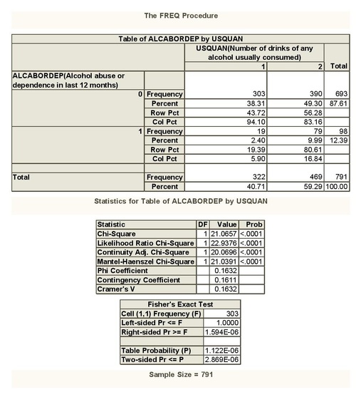
  • Chi-square analysis showed that among daily, or nearly daily, middle adult drinkers the number of drinks (categorical explanatory) is positively and significantly associated with past year DSM-IV alcohol abuse or dependence (categorical response). In fact, corresponding to 1 drink of any alcohol usually consumed (USQUAN=1) we have a total of 5.9% of daily, or nearly daily, middle adult drinkers meeting the criteria for alcohol abuse or dependence; for 2 drinks (USQUAN=2) we have a total of 16.8%; for 3 drinks (USQUAN=3) we have a total of 35.5%; for 8 drinks (USQUAN=8) we have a total of 57.8%. X2 = 256.6, 3 df, p < .0001. That is the more drinks daily, or nearly daily, drinkers drink, the more they are likely to be affected by alcohol abuse or dependence.
  • Moreover, Bonferroni method showed that among daily, or nearly daily, middle adult drinkers the number of drinks is positively and significantly associated with past year DSM-IV alcohol abuse or dependence for each pair of drinking quantity levels with an overall (or family-wise) 95% confidence level, i.e. with an overall type I error rate of 5% (6 comparisons , Bonferroni Adjustment = 0.05 / 6 = 0.008).
  • Daily, or nearly daily, adult drinkers with major depression were significantly more likely to meet the criteria for alcohol abuse or dependence (42%) than those without major depression (24.4%) X2= 37.1, 1 df, p < .0001.


 The following six comparisons are necessary to apply Bonferroni method (Bonferroni Adjustment = 0.05 / 6 = 0.008).


3.3 Moderation


Major depression did not moderate the association between drinking quantity and alcohol abuse or dependence among middle adult drinkers, i.e. drinking quantity is positively and significantly associated with alcohol abuse or dependence for those with major depression (corresponding to 1 drink of any alcohol usually consumed, i.e. USQUAN=1, we have a total of 14.9% of daily, or nearly daily, middle adult drinkers meeting the criteria for alcohol abuse or dependence; for USQUAN=2 have a total of 25.0%; for USQUAN=3 have a total of 50%; for USQUAN=8 have a total of 73.3%) and without major depression (for USQUAN=1 have a total of 3.5%; for USQUAN=2 have a total of 15.2%; for USQUAN=3 have a total of 31.9%; for USQUAN=8 have a total of 52.9%). Moreover, among daily, or nearly daily, middle adult drinkers at each level of drinking the probability of alcohol abuse or dependence was higher among those with major depression than those without major depression.


4 Discussion


4.1 What might the results mean?


  • Drinking quantity is positively and significantly associated with alcohol abuse or dependence among middle adult drinkers both in case they had a major depression at some point in their life and in case they had not.
  • Individuals with major depression seem to be more sensitive to alcohol abuse or dependence across a range of drinking quantity levels.

4.2 Strengths


Results are based on a large nationally representative sample of U.S. middle adults daily, or nearly daily, drinkers.

4.3 Limitations


  • The present findings are based on data collected by observing middle adults daily, or nearly daily, drinkers with and without major depression and they do not show at which drinking quantity levels or drinking frequencies alcohol abuse or dependence emerges, i.e. in case of middle adults drinking less than every day or nearly every day (e.g. 3 to 4 times a week, 2 times a week, etc.)
  • Moreover these findings are based on data collected observing middle adults daily, or nearly daily, drinkers in the past year and do not show drinking quantity levels or drinking frequencies of previous years.

4.4 Recommended Future Research


Further research is needed to determine whether current alcohol abuse or depression in middle adult drinkers may be correlated to high levels of drinking quantity or drinking frequency when such subjects were younger.

5 SAS Source code


                     page 1 / 2


                     page 2 / 2

Monday, May 13, 2013

An application of Cascading Behavior to Political Elections

An application of Cascading Behavior to Political Elections

Gino Tesei - April 24, 2013

This work was born as my peer assignment inside the course of Social Network Analysis by Prof. Lada Adamic, University of Michigan on Coursera. I would like to express my appreciation to Prof. Lada Adamic for the NetLogo model I extended and to the students who review this work for their precious point of view.

Abstract

Political elections are getting hotter and hotter on social networks when such an event occurs. In this work, I consider how new behaviors, practices and conventions can spread new political opinions from person to person through a social network in that case. I focused on two key characteristics of a given social network in case of political elections, i.e. the subjectivity of political issues and the level of resilience inside the network. Hence, two findings are showed. First, higher levels of resilience increases the predictability of political outcome no matter the initial allocation of political opinions. Second, higher levels of variability in payoffs to change opinion decreases the predictability of political outcome.

Part I. Constructing the model

1 Introduction

In [1] Easley and Kleinber considered how new behaviors, practices, opinions, conventions, and technologies spread from person to person through a social network, as people influence their friends to adopt new ideas. The first basic model considered is the so called Networked Coordination Game, where the situation where each node has a choice between two possible behaviors, labeled A and B, is studied. If nodes v and w are linked by an edge, then there is an incentive for them to have their behaviors match:
  • if v and w both adopt behavior A, they each get a payoff of a > 0;
  • if they both adopt B, they each get a payoff of b > 0; and
  • if they adopt opposite behaviors, they each get a payoff of 0.
Suppose that a p fraction of v’s neighbors have behavior A, and a (1 − p) fraction have behavior B, hence it is showed that A is the better choice if p ≥ b ⁄ (a + b). Moreover, it is used the following terminology:
Definition 1 Consider a set of initial adopters who start with a new behavior A, while every other node starts with behavior B. Nodes then repeatedly evaluate the decision to switch from B to A using a threshold of q. If the resulting cascade of adoptionsof A eventually causes every node to switch from B to A, then we say that the set of initial adopters causes a complete cascade at threshold q.
Definition 2 We say that a cluster of density p is a set of nodes such that each node in the set has at least a p fraction of its network neighbors in the set.
Hence the following Claim is proved.
Claim 1 Consider a set of initial adopters of behavior A, with a threshold of q for nodes in the remaining network to adopt behavior A.
(i) If the remaining network contains a cluster of density greater than 1 − q, then the set of initial adopters will not cause a complete cascade.
(ii) Moreover, whenever a set of initial adopters does not cause a complete cascade with threshold q, the remaining network must contain a cluster of density greater than 1 − q.
Hence, the heterogeneous thresholds model is introduced where each node v, we define a payoff av — labeled so that it is specific to v — that it receives when it coordinates with someone on behavior A, and we define a payoff bv that it receives when it coordinates with someone on behavior B.
Finally, the concept of cascade capacity of the network is introduced as the largest value of the threshold q for which some finite set of early adopters can cause a complete cascade. So it is proved that the cascade capacity of the infinite path is at least 1/2 while and there is no network in which the cascade capacity exceeds 1/2 .
Simulating side, the NetLogo model in [2] shows 2 examples from [1] and Lada Adamic Facebook network with the following parameters:
  • payoffs a, b, c > 0 fixed for any node;
  • bilingual option;
  • initial probability blue value.

1.1 Assumptions, parameters, how the model works

Here I will model to the case of political elections, an hot topic on social networks when such an event occurs. Specifically, I’ll build in [3] an extension of model [2] with
  1. heterogeneous thresholds in order to take into account that political issues are subjective and payoffs to change opinion are subjective as well; hence, for each node v, payoffs av = a±ra , with raϵ[-ka, ka] is random and where 0 ≤ ka ≤ a is a futher parameter of the model; on the same way, bv = b±rb with rbϵ[-kb, kb] is random and where 0 ≤ kb ≤ b is a futher parameter of the model;
  2. no bilingual option (= i.e. adopting both A and B), that is not applicable in case of political elections;
  3. % of “resilient” nodes (R) impossible to influence and that never change their initial opinion. This assumption is made to take into account people that, for instance, will vote ever a given party, no matter what their neighbors do.
In order to control the above assumptions, in addition to UI items of NetLogo model in [2], the user has (likewise, in order to get the second point, the bilingual slider has been removed and the related source code commented)
  • the reslience slider (0 to 100) to set up the % of nodes (drawn with the shape of a “cow”) resilient, i.e. that never change their initial opinion no matter what their neighbors think;
  • ka and kb sliders (0 to 100) to set up the maximum payoffs av and bv, so that av = a±ra , with raϵ[-ka, ka] is random and where 0 ≤ ka ≤ a; and bv = b±rb with rbϵ[-kb, kb] is random and where 0 ≤ kb ≤ b.
After such initial setting, the user can
  • choose a network topology among “setup-fb” (Lada Adamic Facebook network), “setup19_4” (a network topology from [1]), “setup19_3” (another network topology from [1]), “setup-line” (line network topology), and
  • allocate opinions,
  • update opinions untill getting an equilibrium.
In order to accomplish the latter step, the user can either use the “alloc-opinion” button after tuning up the initial probability of blue nodes or set up one by one each node as red or blue. It is pobbile to play with a partner with the first person picking one blue node and the second one picking onother red one, and so on. Moreover, the first person can choose a “cow” node (i.e. a resilient node) and, as soon as they are available, the second person can do the same.
Finally, it is possbile to update the color of nodes with the “update” button in order to get start the game. After some hundreds of ticks an equilibrium is typically reached as it can be shown by the following chart.
Hence, I inserted the stop command after 500 ticks. In order to monitor network evolution, the following monitors have been inserted:
  • init-blue: initial number of blue nodes;
  • init-red: initial number of red nodes;
  • resilient-red: number of red cows;
  • resilient-blue: number of blue cows;
  • num-red: number of red nodes;
  • num-blue: number of blue nodes;
  • delta-in / delta-out (ratio): ((num − blue) − (num − red))/((init − blue) − (init − red)).
In the following, I will refer to the ratio delta-in/delta-out just with ratio.
For instance, let suppose we choose se the “setup-fb” with
  • identical payoffs to change opinion, i.e. a = b = 3,
  • probability to have initally A opinion equal to have inially B opinion, i.e. init-blue-prob = 0.5,
  • 34% of persons impossible to influence, i.e. resilience level = 34,
  • no variability in payoffs to change opinion, i.e. ka= kb = 0.
These settings get the following results after simulating elections:
  • init-blue: 76;
  • init-red: 74;
  • resilient-red: 27;
  • resilient-blue: 25;
  • num-red: 106;
  • num-blue: 44;
  • delta-in / delta-out (ratio): -31.
Ceteris paribus (i.e. with the same input parameters), the output ratio can be different. The first question is how much it is different. In order to study statistically this problem, the “100 series” button has been created. By using it, for 100 times NetLogo will
  • setup the Facebook network (setup-fb) with the same input input parameters,
  • allocate and update opinions untill getting an equilibrium.
At the end of such 100 simulations,
  • the monitor “mean” will report the statistical mean of ratio,
  • the monitor “variance” will report the statistical mean of ratio.
  • the monitor “standard deviation” will report the standard deviation of ratio.
The second question is why the ratio can be different starting with the same input parameters. I will answer to this question in the following sections.

1.2 Source Code

Source code can be fully download from [3].

2 An interpretation of the model

The model in [3] is an extension of the one in [2]. Specifically, the model in [3] collapses in the one in [2] by setting
  • 0% of persons impossible to influence, i.e. resilience level = 0,
  • homogeneous payoffs to change political opinion, i.e. ka= kb = 0.
So, we can ask
  1. what kind of impacts we have in the model assuming that a part of nodes (“cows”) are politically resilient to external influence as it happens effectively during political elections?
  2. what kind of impacts we have in the model assuming that nodes have heterogeneous thresholds in order to take into account the subjectivity of political issues (= the payoffs to change opinion are subjective)?
I show an interesting finding. The more the percentage of persons politically resilient to external influence inside the network (“cows”) the less the importance of network topology in order to predict the final political outcome. This can be esily seen thinking at the extreme case, i.e. resilience = 100 corresponding to the case where any node is a “cow”. In that case we would easily predict ratio = 1, i.e. no one will change opinion. In section 3.1 I will show that such a correlation holds in the general case.

Part II. Model testing

3 Misuring two key characteristics of the model

In this section two key characteristics of the model will be measured
  • higher levels of resilience increases the predictability of political outcome no matter the network topology and the initial allocation of red and blue nodes;
  • higher levels of variability in payoffs to change opinion decreases the predictability of political outcome.

3.1 Higher levels of resilience increases the predictability of political outcome no matter the initial allocation of red and blue nodes

In order to study such a problem, I performed the following simulations.
resilience ka kb init-blue-prob. ^mean(ratio) ^variance(ratio) ^std − dev(ratio)
0 0 0 0.5 3.83 899.18 29.98
10 0 0 0.5 3.35 520.49 22.81
20 0 0 0.5 3.60 218.32 14.77
50 0 0 0.5 3.21 111.95 10.58
60 0 0 0.5 2.01 82.29 9.34
70 0 0 0.5 1.42 81.96 9.05
90 0 0 0.5 1.32 13.78 1.94
100 0 0 0.5 0.92 0.07 0.27
A regression of observed mean of ratio has been performed. The value of R2tells us the proportion of the variance in the forecast variable (i.e. the mean of ratio) that can be accounted by the predictor variable (i.e. resilience). Hence, if we know the resilience we can predict 89% of the variability we will see in the mean of ratio. It is a pretty good result (a typical threshold value for R2 is 0.37).
In the same way, if we know the resilience we can predict 72% of the variability we will see in the variance of ratio. It is a pretty good result (a typical threshold value for R2 is 0.37).

3.2 Higher levels of variability in payoffs to change opinion decreases the predictability of political outcome

In order to study such a problem, I performed the following simulations.
resilience ka kb init-blue-prob. ^mean(ratio) ^variance(ratio) ^std − dev(ratio)
0 0 0 0.5 4.46 705.60 26.56
0 10 10 0.5 4.54 731.32 27.04
0 20 20 0.5 2.99 583.03 24.14
0 30 30 0.5 2.27 407.61 20.18
0 40 40 0.5 6.34 429.23 20.71
0 50 50 0.5 6.19 617.39 24.84
0 60 60 0.5 6.64 447.33 21.15
0 80 80 0.5 8.69 424.75 20.61
0 100 100 0.5 5.00 827.24 28.76
Here a regression of observed mean of ratio has been performed. The value of R2tells us the proportion of the variance in the forecast variable (i.e. the mean of ratio) that can be accounted by the predictor variable (i.e. threshold variability ka = kb). Hence, if we know threshold variability we can predict 31% of the variability we will see in the mean of ratio. It is not a good result (a typical threshold value for R2 is 0.37).
In the same way, if we know threshold variability we can predict 0.12% of the variability we will see in the variance of ratio. It is not a good result (a typical threshold value for R2 is 0.37).

4 A comparable existing model chosen and simulated

The comparable existing model chosen is the one in [2], as the model in [3] is an extension of the one in [2]. Specifically, the model in [3] simulates in the one in [2] by setting
  • 0% of persons impossible to influence, i.e. resilience level = 0,
  • homogeneous payoffs to change political opinion, i.e. ka= kb = 0.
I simulated the model in [2] with the one in [3] both in sub-section 3.1 and in sub-section 3.2. For instance, in the former case the following results are produced.
resilience ka kb init-blue-prob. ^mean(ratio) ^variance(ratio) ^std − dev(ratio)
0 0 0 0.5 3.83 899.18 29.98

5 A comparison between two models

The questions that the model in [3] can answer and that the model in [2] can not are
  1. what kind of impacts we have in the model assuming that a part of nodes (“cows”) are politically resilient to external influence as it happens effectively during political elections?
  2. what kind of impacts we have in the model assuming that nodes have heterogeneous thresholds in order to take into account the subjectivity of political issues (= the payoffs to change opinion are subjective)?
At this regard, sub-section 3.1 and 3.2 claim that
  • higher levels of resilience increases the predictability of political outcome no matter the initial allocation of red and blue nodes;
  • higher levels of variability in payoffs to change opinion decreases the predictability of political outcome.

6 Step by step instructions and key points in source code

In this section I will provide
  • step by step instructions for replicating the evaluation; and
  • the related key points in source code.

6.1 Step by step instructions

Download NetLogo model from [3]. Open and set up
  • Facebook network (“setup-fb” button),
  • identical payoffs to change opinion, i.e. a = b = 3,
  • probability to have initally A opinion equal to have inially B opinion, i.e. init-blue-prob = 0.5,
  • 0% of persons impossible to influence, i.e. resilience level = 0,
  • homogeneous payoffs to change political opinion, i.e. ka= kb = 0.
Hence,
  • allocate opinions (“alloc-opinion” button),
  • update opinions (“alloc-opinion” button) untill getting an equilibrium.
On the other side, download NetLogo model from [2]. Open and set up
  • Facebook network (“setup-fb” button),
  • identical payoffs to change opinion, i.e. a = b = 3,
  • probability to have initally A opinion equal to have inially B opinion, i.e. init-blue-prob = 0.5.
Hence,
  • allocate opinions (“alloc-opinion” button),
  • update opinions (“alloc-opinion” button) untill getting an equilibrium.

6.2 Key points in source code

In order to implement resilient nodes (“cows”) and heterogeneous thresholds, the following turtles-own variables must be declared.
turtles-own [   
  resilient   
  a-node ;; heterogeneous payoff    
  b-node ;; heterogeneous payoff  
]
Hence, the update procedure must be properly modified.
...
ask turtles [       
  if resilient = 0 [        
    if any? link-neighbors with [color = blue or color = red] [  
      let payoff-a a-node * count link-neighbors with [color = blue]
      let payoff-b b-node * count link-neighbors with [color = red] 
      set color blue       
      if (payoff-a < payoff-b) [            
        set color red          
      ]          
      if ((payoff-a = payoff-b) and (random 100 < 50)) [
        set color red    
      ]        
    ]     
]     ]    
​
...
​
tick
...
For other minor modifications, please refer to source code from [3].

Part III. Interpretation

7 Limitations of data

The main limitation is that conclusions of sub-section 3.1 and 3.2 are derived from a single network topology (Lada Adamic Facebook network). In order to extend such conclusions to the general case, simulations and related regressions of sub-section 3.1 and 3.2 should be performed in a wider range of network topologies.
Another limitations is that conclusions of sub-section 3.1 and 3.2 are derived starting from a statistically initial equal situation (i.e. initial number of red nodes statistically equal to the number of initial blue nodes). In order to extend such conclusions to the general case, simulations and related regressions of sub-section 3.1 and 3.2 should be performed in a wider range of inital political allocation patterns.

8 Insights from the analysis

Conclusions of sub-section 3.1 and 3.2 claim that
  • higher levels of resilience increases the predictability of political outcome no matter the network topology and the initial allocation of red and blue nodes;
  • higher levels of variability in payoffs to change opinion decreases the predictability of political outcome.
Hence,
  • samples of social network comminities could be studied in order to asses the level of political resilience (e.g. members can answer to some questionaries). If such a level is high (e.g. forums where people have same political opinions), then the model could be used in order to predict and influence political outcome inside that community (e.g. putting strategically some “cows” inside the network).
  • samples of social network comminities could be studied in order to asses the level of variability in payoffs to change political opinion (e.g. members can answer to some questionaries). If such a level is high, we know is very hard to influence and predict political outcome inside the whole community. A strategy could be trying to cut the community (e.g. putting strategically some “cows” around weak ties of community) and repeat the process on the two seprate communities.

References

[1] Easley and Kleinberg, Networks, Crowds and Markets, Ch19.Cascading Behavior in Networks
[3] Gino Tesei, NetLogo Model for political elections (https://docs.google.com/file/d/0B1zSgDfZgjLTY1REdjZlR3JCcU0/edit?usp=sharing)

Saturday, February 09, 2013

Will users' awareness of Facebook inability to protect privacy be the Facebook killer?


Facebook monthly active users (MAUs) were 1.06 billion as of December 31 2012. The company noted that now stores over 100 petabytes of media (photos and videos). Hence, each Facebook user needs on average almost 100 Mbyte for photos and videos. In addiction, there's data necessary for personal user profile information, but as it's text based it's likely to be some size level lower. 

A great deal of data. But why does Facebook business model need so much data? "Our goal is to help every person stay connected and every product they use be a great social experience," Mark Zuckerberg says. In fact, Facebook business model is focused On Line Adverstising, payments and other fees (aka virtual goods; e.g. fees from games). Sandberg also views local businesses as a growth opportunity for the company. "Local is the holy grail of the Internet, but local businesses are not very tech savvy. More than 40 percent have no Web presence at all. Facebook has a huge competitive advantage because they are using Facebook personally, and seeing messages from other businesses," she said. "It's a smaller leap (to use Facebook), and the numbers bear that out -- 7 million small businesses are using Facebook Pages on a monthly basis, and hundreds of thousands are upsold to become advertisers."  

Average Revenue per User (ARPU) Q2'12 was $1.28 with some differences:
  • US & Canada: $3.20 
  • Europe: $1.43
  • Asia: $0.55
  • Rest of the world: $0.44
Q2'12 revenue totaled $1.18 billion, an increase of 32%, compared with $895 million of Q2'11:
  1. Revenue from advertising was $992 million, representing 84% of total revenue and a 28% increase from the same quarter last year.
  2. Payments and other fees revenue for the second quarter was $192 million
This revenue structure is rather consilidated as full year 2012 results shows:
  • 84% revenue from adv
  • 16% revenue from payments and other fees.
Interesting that mobile revenue represented approximately 23% of advertising revenue for Q4'12 up from 14% Q3'12. Globally, 2012 revenue increased 27% up to $5.089 billions from $3.711 billions of 2011.

Different music on operating margin & net income side.   2012 (non-GAAP) income from operations decreased to $538 millions from  $1.756 billions of 2011. Looking at the main costs and expenses:
  • Research and development (+261% vs 2011): $1.399 mln 
  • Marketing and sales (+128% vs 2011): $896 mln   
  • General and administrative  (+184% vs 2011): $892 mln
Facebook is obviously investing heavily on R&D , MKTG & Sales and it's completing its expansion. So, the 2012 net income shouldn't be interesting (!!!). Actually, 2012 net income is $53 mln vs $1 billion of 2011 (before IPO). That's a clear sign that Facebook is a long term investment and not a speculative bet for extempore investors, but that's not the point here. The point is that Facebook went public to get the necessary resources do do these technology/product/corporate investments and developing a unique competitive avdantage (Facebook MAUs are actually unique!) and how the return could be affected by the untechnological factor of users' awareness of Facebook inability to protect privacy.

Where is Facebook investing and where it can get a unique advantage?
  • Big Data (for final users: search, social graph search, recommendation engine, etc.; for clients: Sentiment Analysis, Marketing Campaign Analysis, Customer Churn Analysis, Customer Experience Analytics, etc.)
  • Mobile support & integration (iOS, Andrioid, etc.)
  • Product development (Messenger for Android and iOS, Facebook Camera available in 18 languages, new advertising products such as Custom Audiences, Facebook Exchange, Offers, and mobile app install ads, Created Facebook Stories, global App Center, etc. ) 
  • Corporate development (first international engineering office in London, etc.)
Talking about product, Google+ is considered actually a better product by someone, but unluckily Google+ hasn't the Facebook MAUs. I think MAUs and its exploitation is the core asset Facebook can use to get a unique competitive advantage over competitors and get satisfactory return to investors.   

Talking about MAUs explotation, technologies behind Big Data are
  • Hadoop & related fameworks (Hadoop Distributed File System, MapReduce, Hive, Pig, HBase, Flume, Oozie, Flume, Ambari, Avro, Mahout, Sqoop, HCatalog, BigTop, etc.),  
  • NoSQL databases (HBase, Cassandra, Aerospike, MongoDB, Accumulo, Riak, CouchDB, DynamoDB, etc.). 
Effectively, some of these technologies were initially developed in Google and Facebook. Now, they most live as open source projects and applied by Facebook in order to make applications / services interesting for Facebook users/clients, such as:
  • Recommendation Engine: Web properties and online retailers use Hadoop to match and recommend users to one another or to products and services based on analysis of user profile and behavioral data. LinkedIn uses this approach to power its “People You May Know” feature, while Amazon uses it to suggest related products for purchase to online consumers. Initial question turns here into the following one: how users' awareness of Facebook inability to protect privacy can prevent users to recommend some kinds products or users? Is there particular products or relationships between users more sensitive than others? 
  • Sentiment Analysis: Used in conjunction with Hadoop, advanced text analytics tools analyze the unstructured text of social media and social networking posts, including Tweets and Facebook posts, to determine the user sentiment related to particular companies, brands, products or politic parties. Analysis can focus on macro-level sentiment down to individual user sentiment. Initial question turns here into the following one: how users' awareness of Facebook inability to protect privacy can prevent users to express their opinion about companies, brands or products? Is there particular companies, brands, products or politic parties more sensitive than others? 
  • Social Graph Analysis: In conjunction with Hadoop and NoSQL databases, social networking data is mined to determine which customers pose the most influence over others inside social networks. This helps enterprises determine which are their “most important” customers, who are not always those that buy the most products or spend the most but those that tend to influence the buying behavior of others the most. how users' awareness of Facebook inability to protect privacy can prevent users to influence others users? Is here particular companies, brands, products, political issues or arguments more sensitive than others?
A Final metaphor 
In information theory, the Shannon–Hartley theorem tells the maximum rate at which information can be transmitted over a communications channel of a specified bandwidth in the presence of noise.


        C =  B \log_2 \left( 1+\frac{S}{N} \right)

where C is the channel capacity (bits per second), B is the bandwidth of the channel (hertz), S is the average received signal power over the bandwidth, N is the average noise or interference power over the bandwidth (watts), S/N is the signal-to-noise ratio (SNR). Hence, the more the noise power, the more the signal power necessary to get a given capacity. Or, fixed the signal power, the more the  noise power, the less the channel capacity.   

Perhaps, we can think the channel capacity (C) as the value delivered to Facebook clients by services such as Recommendation Engine, Sentiment Analysis or Social Graph Analysis; the signal power (S) as the effectiveness of Big Data technology in order to discover such information; the noise power (N) as the interference because of users' awareness of Facebook inability to protect privacy in letting users having a full social experience; the bandwidth (B) as the Facebook MAUs. 

Hence, if that metaphor works, given Facebook MAUs, the more the users' awareness of Facebook inability to protect privacy, the more the effectiveness of Big Data technology to get the same value to clients, the more R&D investments, the higher the price for Facebook clients ... the less the likelihood that Facebook business model works... 

Sunday, February 03, 2013

WSJ: Big Data Pay Premium ‘Highest It Will Ever Be’

According to a January report from the IT research firm Foote Partners LLC, which gathered compensation data from 2,435 employers. For example, expertise in Hadoop and Cassandra, platforms capable of processing massive amounts of unstructured data like feeds from social media, commanded pay premiums of up to 16% and 14% respectively. 


Friday, January 25, 2013

A simple way for data cleaning in VBA Excel

In data analysis data cleaning is the act of detecting and either removing or correcting inaccurate records from a record set. In case data is fetched from a Data Base Relational Systems, we're talking about incorrect or inaccurate records from a table.  For instance, in Excel 2007+ you can fetch data from a DBMS such as SQL Server in the Get External Data group. The following step is removing or correcting inaccurate records. A typical way to do it is scanning the Excel data sheet following from the top and from left to rigth, processing only columns storing data validity information. Hence, you need a VBA function such as the following:

clean("FromSheet", "ToSheet", CellCondition, Condition, True)

i.e. a VBA function with a signature like

Function clean(FromSheet As String, ToSheet As String, CellCondition As Variant, Condition As Variant, Caption As Boolean) As Long   


A typical safe way to implement such a action is copying in a new sheet the clean data. That works especially in case you refresh data sheet periodically from an external data source. Here's the VBA code. 


    Set wsI = Sheets(FromSheet)
    Set wsO = Sheets(ToSheet)

    LastRow = wsI.Range("A" & Rows.Count).End(xlUp).Row
   
    j = 1
    With wsI
        For i = 1 To LastRow
           
            ok = False
             For N = LBound(CellCondition) To UBound(CellCondition)
                 If Trim(.Range(CellCondition(N) & i).Value) = Condition(N) Then
                     ok = True
                 End If
             Next N
       
            If Caption And i = 1 Then
                ok = True
            End If
           
            If ok Then
                wsI.Rows(i).Copy wsO.Rows(j)
                j = j + 1
            End If
           
        Next i
    End With